Introducing op_pandas
pandas is a fast, powerful, flexible and easy to use open source data analysis and manipulation tool, built on top of the Python programming language.
We have created a differentially private version of pandas library named op_pandas. This lets you handle private dataframes and private series which can be used to perform various statistical analysis with differential privacy guarantees. The api methods have been created such that it gives you minimal difficulty from getting adjusted if you have used pandas before.
Getting Started: Install, Import & Connect to Antigranular
!pip install antigranular
import antigranular as ag
session = ag.login("<ag client secrets>", "<ag client secrets>", competition = "Sandbox Competition")
>>> Loading dataset "Medical Treatment" to the kernel...
Dataset "Medical Treatment" loaded to the kernel as medical_treatment
Connected to Antigranular server session id: 66b9293d-ecb6-4059-ac24-c8fe2afb3b4f, the session will time out if idle for 60 minutes
Cell magic '%%ag' registered successfully, use `%%ag` in a notebook cell to execute your python code on Antigranular private python server
🚀 Everything's set up and ready to roll!
This is a short introduction to op_pandas (Oblivious private pandas), geared mainly for new users. Let's get started! You can import the library as follows:
%%ag
from op_pandas import PrivateDataFrame , PrivateSeries
Object Creation
From AG-Server
To load a dataset from AG-Server and obtain the required data structures, you can use the load_dataset() function from ag_utils. The response of the load_dataset() function provides the necessary data in a dictionary format.
%%ag
"""
medical treatment dictionary :-
{
  "train_x": pdf_train_x,
  "train_y": pdf_train_y,
  "test_x": df_test_x,
}

These are Private datastructures and cannot be exported to local environment.
Unless a differentially private measure is applied to obtain a non-private
DataFrame or Series.
"""
train_x = medical_treatment["train_x"]
train_y = medical_treatment["train_y"]
test_x = medical_treatment["test_x"]
From pandas.Series
When creating a PrivateSeries, it's recommended to set metadata bounds. This allows you to define the range of valid values for the series. If you don't provide explicit bounds, op_pandas will automatically assign the metadata based on the minimum and maximum values in the series.
%%ag
import pandas as pd
s = pd.Series([1,5,8,2,9] , name='Test_series')
priv_s = PrivateSeries(series=s,metadata=(0,10))
From pandas.DataFrame
Similar to PrivateSeries, it's recommended to set metadata bounds when creating a PrivateDataFrame. By specifying metadata, you can define the valid range of values for each column in the dataframe. If metadata bounds are not provided, op_pandas will assign automatic bounds based on the minimum and maximum values in each numerical column.
%%ag
import pandas as pd
data = {
    'Age':[20,30,40,25,30,25,26,27,28,29],
    'Salary':[35000,60000,100000,55000, 35000,60000,100000,55000,35000,60000],
    'Sex':['M','F','M','F', 'M','F','M','F', 'M', 'F']
}
metadata = {
    'Age':(18,65),
    'Salary':(20000,200000)
}
df = pd.DataFrame(data)
priv_df = PrivateDataFrame(df=df , metadata=metadata)
Importing data
Within the AG environment, we can also import external data from local jupyter session.
import pandas as pd
import numpy as np
import string, random

arr_name = []
n_num = 10000
N = 10
for i in range(n_num):
  res = ''.join(random.choices(string.ascii_lowercase, k=N))
  arr_name.append(res)

df = pd.DataFrame({'name': arr_name, 'age': np.random.randint(0, 80, n_num), 'salary': np.random.randint(100, 100000, n_num)})

session.private_import(data = df, name= 'imported_df')
>>> dataframe cached to server, loading to kernel...
# Creating another dataset with NaNs in it

# Randomly distributing nans in two columns with prob = 0.5

choice = [1,2,np.nan]
a = np.random.choice(choice,10000,p=[0.25,0.25,0.5])
b = np.random.choice(choice,10000,p=[0.25,0.25,0.5])

df_2 = pd.DataFrame({'a': a, 'b': b})

session.private_import(data = df_2, name = "imported_df_2")
>>> dataframe cached to server, loading to kernel...
Output: Dataframe loaded successfully to the kernel
After using private_import, you can access the dataFrame with the name imported_df within the AG environment. We will create a PrivateDF out of it.
%%ag
metadata = {
    'age': (0, 80),
    'salary': (1, 200000)
}

priv_df = PrivateDataFrame(imported_df ,metadata = metadata)
>>> Dataframe loaded successfully to the kernel
Viewing Data
To protect privacy, records in PrivateDataFrame and PrivateSeries cannot be viewed directly. However, you can still analyse and obtain statistical information about the data using methods that offer differential privacy guarantees.
Viewing details about the data
Printing the details about the data, like columns and metadata can be done in the following way:
%%ag

ag_print("Columns: \n", priv_df.columns)
ag_print("Metadata: \n", priv_df.metadata)
ag_print("Dtypes: \n", priv_df.dtypes)
>>> Columns:
 Index(['name', 'age', 'salary'], dtype='object')
Metadata:
 {'age': (0, 80), 'salary': (1, 200000)}
Dtypes:
 name      object
age        int64
salary     int64
dtype: object
Quick Statistics
One way to obtain the quick-statistic is by using the describe() method where you can spend some epsilon to obtain a rough meta-data about the dataset.
%%ag

priv_describe = priv_df.describe(eps=1)
# Export information from remote ag kernel to local jupyter server.
ag_print(priv_describe)
>>>
                age         salary
count  10011.000000   10011.000000
mean      39.430439   49728.643224
std       23.065769   28405.891863
min        0.000000     583.443063
25%       19.904847   24461.587152
50%       35.801599   50159.255936
75%       60.452492   74499.712660
max       77.701005  147580.823075
You can view the statistics by exporting the non-private result to the local Jupyter server:
%%ag

export(priv_describe, name='priv_describe')
Setting up exported variable in local environment: priv_describe
print(priv_describe)
>>>
                age         salary
count  10011.000000   10011.000000
mean      39.430439   49728.643224
std       23.065769   28405.891863
min        0.000000     583.443063
25%       19.904847   24461.587152
50%       35.801599   50159.255936
75%       60.452492   74499.712660
max       77.701005  147580.823075
Cleaning Data
You can use dropna method to remove any records that contain nan values in any of its features.
Cleaning using dropna method.
%%ag
# probability of a record not having nan = (0.5 * 0.5) = 0.25
# Hence expected count after dropna should be around 2500.
priv_df_2 = PrivateDataFrame(imported_df_2, metadata = {'a': (1, 2), 'b': (1, 2)})

export(priv_df_2.dropna(axis=0).describe(eps=1), 'result')
>>> Setting up exported variable in local environment: result


/code/dependencies/op_pandas/op_pandas/core/private_dataframe.py:115: SettingWithCopyWarning:
A value is trying to be set on a copy of a slice from a DataFrame

See the caveats in the documentation: https://pandas.pydata.org/pandas-docs/stable/user_guide/indexing.html#returning-a-view-versus-a-copy
  self._df[col].clip(lower=self._metadata[col][0], upper=self._metadata[col][1], inplace=True)
print(result)
>>>
                 a            b
count  2490.000000  2490.000000
mean      1.495172     1.502561
std       0.496467     0.483317
min       1.000000     1.000000
25%       1.000000     1.000000
50%       1.264635     1.668942
75%       1.985666     1.975653
max       1.997052     1.993214
print(df_2.dropna(axis=0).describe())
>>>
                 a            b
count  2490.000000  2490.000000
mean      1.492369     1.503213
std       0.500042     0.500090
min       1.000000     1.000000
25%       1.000000     1.000000
50%       1.000000     2.000000
75%       2.000000     2.000000
max       2.000000     2.000000
We can also drop some columns from the PrivateDataFrame using drop functionality.
%%ag
ag_print("Columns before: ", priv_df.columns)

temp_df = priv_df.drop(['name'], inplace = False)

ag_print("Columns After Dropping name: ", temp_df.columns)
>>> Columns before:  Index(['name', 'age', 'salary'], dtype='object')
Columns After Dropping name:  Index(['age', 'salary'], dtype='object')
Selecting Data
Setting values that affect a certain set of records is not allowed in PrivateDataFrame or PrivateSeries. However, you can apply transformation functions using PrivateDataFrame.ApplyMap or PrivateSeries.Map.
Getting Data Objects
To select a single column and obtain a PrivateSeries, equivalent to df["A"]:
%%ag

priv_s = priv_df['age']
ag_print("Describe:\n", priv_s.describe(eps=1))
ag_print("Metadata:\n", priv_s.metadata)
>>> Describe:
 count    9988.000000
mean       39.472473
std        22.735391
min         0.000000
25%        21.384668
50%        37.840602
75%        55.273188
max        78.730881
Name: series, dtype: float64
Metadata:
 (0, 80)
To select a collection of columns which returns a PrivateDataFrame
%%ag

priv_df_filtered = priv_df[['age','salary']]

ag_print("Columns:\n", priv_df_filtered.columns)
ag_print("Metadata:\n", priv_df_filtered.metadata)
>>> Columns:
 Index(['age', 'salary'], dtype='object')
Metadata:
 {'age': (0, 80), 'salary': (1, 200000)}


/code/dependencies/op_pandas/op_pandas/core/private_dataframe.py:115: SettingWithCopyWarning:
A value is trying to be set on a copy of a slice from a DataFrame

See the caveats in the documentation: https://pandas.pydata.org/pandas-docs/stable/user_guide/indexing.html#returning-a-view-versus-a-copy
  self._df[col].clip(lower=self._metadata[col][0], upper=self._metadata[col][1], inplace=True)
Setting Data Objects
Setting any values that affect a record is not allowed in PrivateDataFrame or PrivateSeries. However, you can apply transformation functions using PrivateDataFrame.ApplyMap or PrivateSeries.Map
Using Applymap on a PrivateDataFrame
%%ag


# maps string to its length if not numerical else divides it by 2.
def func(x: str | int | float) -> float:
    if isinstance(x, str):
        return len(x)
    elif isinstance(x, (int, float)):
        return x / 2
    return 0.0


result = priv_df.applymap(func, eps=1)
%%ag
ag_print("Metadata:\n", result.metadata)
ag_print("Describe:\n", result.describe(eps = 1))
>>> Metadata:
 {'name': (8.0, 16.0), 'age': (0.0, 64.0), 'salary': (512.0, 65536.0)}

Describe:
                name           age        salary
count  10001.000000  10001.000000  10001.000000
mean       9.979915     19.763231  25068.695612
std        0.274668     10.477926  16333.537130
min        8.000000      0.000000    686.474307
25%       10.000000      8.740750  12489.945476
50%       10.000000     18.864365  24417.320448
75%       10.000000     28.283437  37265.078587
max       10.000000     35.126989  60705.413286
## Calculating the original results

def func(x: str | int | float) -> float:
    if isinstance(x, str):
        return len(x)
    elif isinstance(x, (int, float)):
        return x / 2
    return 0.0

result_local = df.applymap(func)
print("Describe: ", result_local.describe())
>>>
Describe:            name           age        salary
count  10000.0  10000.000000  10000.000000
mean      10.0     19.720800  24840.119300
std        0.0     11.544976  14512.035948
min       10.0      0.000000     50.500000
25%       10.0      9.500000  12210.250000
50%       10.0     19.500000  24811.750000
75%       10.0     30.000000  37367.750000
max       10.0     39.500000  49993.000000
Using Map on a PrivateSeries. The mapping can be done either via using a dictionary for 1:1 mapping or via a callable method.
%%ag

def series_map(x:int)->float:
    return x/2

priv_df['age'] = priv_df['age'].map(series_map,eps=1) # important
ag_print("Metadata:\n", priv_df.metadata)
>>> Metadata:
 {'age': (0.0, 64.0), 'salary': (1, 200000)}
Operations
This section covers various operations that can be performed on PrivateDataFrame and PrivateSeries objects.
Unary Ops
You can perform unary operations such as ~, -, +, and abs on PrivateDataFrames and PrivateSeries. These operations apply element-wise to the data.
The ~ operator performs the bitwise negation operation.
The - operator performs the arithmetic negation operation.
The + operator performs the arithmetic addition operation.
The abs() function calculates the absolute value of each element.
%%ag

export(priv_df_2.describe(eps=2) , 'original')
export((-priv_df_2).describe(eps=2) , 'negative')
>>> Setting up exported variable in local environment: original
Setting up exported variable in local environment: negative
negative.columns = ["a_neg","b_neg"]
print(original.join(negative , how="left"))
>>>
                  a             b         a_neg         b_neg
count  10000.000000  10000.000000  10000.000000  10000.000000
mean       1.498597      1.504388     -1.500690     -1.503697
std        0.494197      0.498858      0.498402      0.499788
min        1.000000      1.000000     -1.000000     -1.000000
25%        1.000000      1.000000     -1.001932     -1.001540
50%        1.635791      1.891447     -1.678784     -1.161680
75%        1.991538      1.997409     -1.996417     -1.996500
max        1.992424      1.997140     -1.999776     -1.999894
Binary Ops
Similar to pandas.DataFrame , you can apply binary operations using scalars and PrivateDataFrames against PrivateDataFrames.
Binary operations on a mix of scalars and PrivateDataFrames against PrivateDataFrames.
%%ag

pdf = priv_df[['age','salary']]
result1 = pdf + (10*pdf)  # expected min-max => Age:(0,704) ,  Salary:(11, 2200000)
result2 = result1/1000 # expected min-max => Age:(0,0.704) ,  Salary:(0.011, 2200)
ag_print("Result1 metadata: \n", result1.metadata)
ag_print("Result2 metadata: \n", result2.metadata)
>>> Result1 metadata:
 {'age': (0.0, 704.0), 'salary': (11, 2200000)}
Result2 metadata:
 {'age': (0.0, 0.704), 'salary': (0.011, 2200.0)}


/code/dependencies/op_pandas/op_pandas/core/private_dataframe.py:115: SettingWithCopyWarning:
A value is trying to be set on a copy of a slice from a DataFrame

See the caveats in the documentation: https://pandas.pydata.org/pandas-docs/stable/user_guide/indexing.html#returning-a-view-versus-a-copy
  self._df[col].clip(lower=self._metadata[col][0], upper=self._metadata[col][1], inplace=True)
Bitwise Ops
Similar to pandas.DataFrame, you can apply bitwise operations using scalars and PrivateDataFrames against PrivateDataFrames. These operations apply element-wise to the data.
%%ag
import numpy as np
import pandas as pd

priv_ser_1 = PrivateSeries(pd.Series(np.random.randint(0,1,10000)), metadata=(0,1))
priv_ser_2 = PrivateSeries(pd.Series(np.random.randint(0,1,10000)), metadata=(0,1))

"""
{
    priv_ser_1 : randomly sampled integer data containing (0,1)
    priv_ser_1 : randomly sampled integer data containing (0,1)
}
"""

ag_print("Describe of private Series 1: \n", priv_ser_1.describe(eps = 1))
ag_print("Describe of private Series 2: \n", priv_ser_2.describe(eps = 1))

result = priv_ser_1 & priv_ser_2

ag_print("Describe of the result: \n", result.describe(eps = 1))
>>> Describe of private Series 1:
 count    9.998000e+03
mean     1.571300e-03
std      1.998231e-02
min      0.000000e+00
25%      4.656613e-10
50%      4.656613e-10
75%      4.656613e-10
max      4.656613e-10
Name: series, dtype: float64

Describe of private Series 2:
 count    1.000500e+04
mean     5.608570e-04
std      4.612496e-02
min      0.000000e+00
25%      4.656613e-10
50%      4.656613e-10
75%      4.656613e-10
max      4.656613e-10
Name: series, dtype: float64

Describe of the result:
 count    1.000700e+04
mean     3.952059e-04
std      2.277582e-02
min      0.000000e+00
25%      4.656613e-10
50%      4.656613e-10
75%      4.656613e-10
max      4.656613e-10
Name: series, dtype: float64
General Functions
op_pandas comes packaged with some useful functions like to_datetime, concat, merge and train_test_split.
Concat
Let us create a copy of priv_df and concatenate the copy with the original.
arr_name = []
n_num = 10000
N = 10
for i in range(n_num):
  res = ''.join(random.choices(string.ascii_lowercase, k=N))
  arr_name.append(res)

df = pd.DataFrame({'name': arr_name, 'age': np.random.randint(0, 80, n_num), 'salary': np.random.randint(100, 100000, n_num)})

session.private_import(data = df, name= 'imported_df_copy')
>>> dataframe cached to server, loading to kernel...
Output: Dataframe loaded successfully to the kernel
%%ag
metadata = {
    'age': (0, 80),
    'salary': (1, 200000)
}

priv_df_copy = PrivateDataFrame(imported_df_copy ,metadata = metadata)
%%ag

ag_print("First DF count:\n",priv_df.count(eps = 1))
ag_print("Second DF count:\n",priv_df_copy.count(eps = 1))

import op_pandas
concat_df = op_pandas.concat([priv_df, priv_df_copy])
ag_print("Concat DF count: \n", concat_df.count(eps=1))
>>> First DF count:
 name      10000
age        9999
salary     9988
dtype: int64

Second DF count:
 name       9998
age        9999
salary    10001
dtype: int64

Concat DF count:
 name      19997
age       20000
salary    20004
dtype: int64
We can only use concat to concatenate over indices.
Keep in mind that the datatypes of same columns for all dataframes must be same.
Train_test_split
We can use op_pandas.train_test_split to create train and test splittings of a PrivateDataFrame/Series or an array of PrivateDataFrames/Series.
%%ag

priv_df_train, priv_df_test = op_pandas.train_test_split(priv_df)

ag_print("Count of train split:\n",priv_df_train.count(eps = 1))
ag_print("Count of test split:\n",priv_df_test.count(eps = 1))
>>> Count of train split:
 name      7501
age       7503
salary    7500
dtype: int64

Count of test split:
 name      2492
age       2499
salary    2491
dtype: int64
JOINS and WHERE
This section explores different operations related to joining PrivateDataFrame and PrivateSeries objects and using the WHERE and JOIN method for filtering data.
JOIN on Private objects
Joining two PrivateDataframes:
%%ag
"""
pdf: {randomly sampled}
    columns = ['A','B','C']
    metadata = (0,100) for all columns
    size = 1000

pdf2: {randomly sampled}
    columns = ['E','F']
    metadata = (-100,100) for all columns
    size = 1000

ps: {randomly sampled series}
    name = 'series'
    metadata = (0,100)
    size = 1000
"""

pdf = PrivateDataFrame(pd.DataFrame({"A": np.random.randint(0,100,1000), "B": np.random.randint(0,100,1000), "C": np.random.randint(0,100,1000)}), metadata = {"A": (0, 100), "B": (0, 100), "C": (0, 100)})
pdf2 = PrivateDataFrame(pd.DataFrame({"E": np.random.randint(-100,100,1000), "F": np.random.randint(-100,100,1000)}), metadata = {"E": (-100, 100), "F": (-100, 100)})
ps = PrivateSeries(pd.Series(np.random.randint(0,100,1000)), metadata=(0,100))
%%ag #join with dataframe
result = pdf.join(pdf2,how="outer")
ag_print("Outer Join of two PDFs Describe:\n",result.describe(eps=1))
>>> Outer Join of two PDFs Describe:
                 A           B           C           E           F
count  978.000000  978.000000  978.000000  978.000000  978.000000
mean    45.078161   48.373313   47.395728    2.918509    0.379322
std     41.659230   39.782047    3.978732   55.174294   76.570248
min      0.000000    0.000000    0.000000 -100.000000 -100.000000
25%     25.835038   16.814188   13.689315  -55.716763  -79.960320
50%     45.534085   55.195066   57.023430    3.266460   -5.226773
75%     62.600983   63.868197   68.137527   40.907116   58.650339
max     93.493320   94.355744   79.755250   58.467962   89.288805
Joining PrivateDataframe with PrivateSeries:
%%ag # join with series
result = pdf.join(ps,how="inner")
ag_print("Inner Join of PDF and Series Describe:\n",result.describe(eps=1))
>>> Inner Join of PDF and Series Describe:
                 A           B           C      series
count  995.000000  995.000000  995.000000  995.000000
mean    50.461822   50.737590   44.956548   52.693788
std     28.974945   35.573564   28.876807   39.639266
min      0.000000    0.000000    0.000000    0.000000
25%     11.820072   43.155183   48.520076    8.472153
50%     65.126290   35.547530   28.150633   60.640127
75%     89.179010   85.479518   50.462041   68.068637
max     97.001126   79.362787   92.063356   75.326474
WHERE Query
%%ag

result = pdf.where(pdf > 0)
ag_print("Where Query Result:\n", result.describe(eps=1))
>>> Where Query Result:
                  A            B            C
count  1001.000000  1001.000000  1001.000000
mean     48.506532    50.754384    53.904313
std      42.434438    24.036048    27.686005
min       0.000000     0.000000     0.000000
25%      23.367422    21.512664     4.402222
50%      33.757446    52.456891    22.643254
75%      65.482272    81.311059    74.171133
max      92.626234    84.918578    98.803625
Statistical Methods
PrivateDataframe and PrivateSeries also support wide range of statistical methods with similar api of that to pandas.DataFrame and pandas.Series.
sum,mean,countstd,varquantile,percentile,median- bounded min and max can be achieved using
percentile(0)andpercentile(100)respectively histandhist2dcov(covariance),skew(skewness),corr(correlation)
Basic Statistics
This example demonstrates the usage of differentially private variance and count methods on a PrivateSeries.
The resulting values are differentially private while providing statistical insights about the data.
%%ag
var = ps.var(eps = 1)
count = ps.count(eps = 1)

ag_print(f"variance = {var} , count = {count}")
>>> variance = 806.7200376847192 , count = 1000
You can find differentially private bounded max and min using the percentile method.
%%ag

min = ps.percentile(eps=0.1 ,p = 0)
max = ps.percentile(eps=0.1 , p =100)
ag_print(f"min = {min} , max = {max}") ## Actual min, max : (0,100)
>>> min = 3.7421055945821973 , max = 99.09590214840338
Advanced Statistics
You can perform more complex differentially private statistical calculations like covariance, skewness, and correlation similar to their counterparts in pandas. Finding correlation matrix of a PrivateDataFrame and comparing the results with the original expected result.
%%ag

result = priv_df.corr(eps=3)
export(result,'private_result')
>>> Setting up exported variable in local environment: private_result
print(private_result)
>>>             age    salary
age          1.0  0.032151
salary  0.032151       1.0
print(df[['age', 'salary']].corr())
>>>             age    salary
age     1.000000  0.006333
salary  0.006333  1.000000
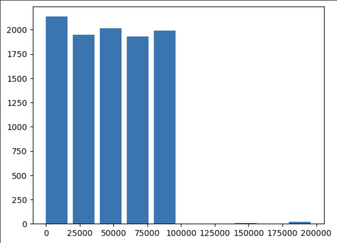
Histograms
You can generate differentially private histograms using PrivateDataFrame.hist().
%%ag

hist_data = priv_df.hist(column='salary',eps=0.1)
export(hist_data , 'hist_data')
>>> Setting up exported variable in local environment: hist_data
To visualise the histogram locally, you can use matplotlib or any other plotting library of your choice.
import matplotlib.pyplot as plt
dp_hist, dp_bins = hist_data
# Create a bar plot using Matplotlib
plt.bar(dp_bins[:-1], dp_hist, width=np.diff(dp_bins)*0.8, align='edge')

# Display the plot
plt.show()
Now that we are all done, we can terminate the session. Happy coding!
session.terminate_session()
>>> {'status': 'ok'}